Robust Linear Models
[1]:
%matplotlib inline
[2]:
import matplotlib.pyplot as plt
import numpy as np
import statsmodels.api as sm
Estimation
Load data:
[3]:
data = sm.datasets.stackloss.load()
data.exog = sm.add_constant(data.exog)
Huber’s T norm with the (default) median absolute deviation scaling
[4]:
huber_t = sm.RLM(data.endog, data.exog, M=sm.robust.norms.HuberT())
hub_results = huber_t.fit()
print(hub_results.params)
print(hub_results.bse)
print(
    hub_results.summary(
        yname="y", xname=["var_%d" % i for i in range(len(hub_results.params))]
    )
)
const       -41.026498
AIRFLOW       0.829384
WATERTEMP     0.926066
ACIDCONC     -0.127847
dtype: float64
const        9.791899
AIRFLOW      0.111005
WATERTEMP    0.302930
ACIDCONC     0.128650
dtype: float64
                    Robust linear Model Regression Results
==============================================================================
Dep. Variable:                      y   No. Observations:                   21
Model:                            RLM   Df Residuals:                       17
Method:                          IRLS   Df Model:                            3
Norm:                          HuberT
Scale Est.:                       mad
Cov Type:                          H1
Date:                Tue, 14 May 2024
Time:                        16:34:08
No. Iterations:                    19
==============================================================================
                 coef    std err          z      P>|z|      [0.025      0.975]
------------------------------------------------------------------------------
var_0        -41.0265      9.792     -4.190      0.000     -60.218     -21.835
var_1          0.8294      0.111      7.472      0.000       0.612       1.047
var_2          0.9261      0.303      3.057      0.002       0.332       1.520
var_3         -0.1278      0.129     -0.994      0.320      -0.380       0.124
==============================================================================

If the model instance has been used for another fit with different fit parameters, then the fit options might not be the correct ones anymore .
Huber’s T norm with ‘H2’ covariance matrix
[5]:
hub_results2 = huber_t.fit(cov="H2")
print(hub_results2.params)
print(hub_results2.bse)
const       -41.026498
AIRFLOW       0.829384
WATERTEMP     0.926066
ACIDCONC     -0.127847
dtype: float64
const        9.089504
AIRFLOW      0.119460
WATERTEMP    0.322355
ACIDCONC     0.117963
dtype: float64
Andrew’s Wave norm with Huber’s Proposal 2 scaling and ‘H3’ covariance matrix
[6]:
andrew_mod = sm.RLM(data.endog, data.exog, M=sm.robust.norms.AndrewWave())
andrew_results = andrew_mod.fit(scale_est=sm.robust.scale.HuberScale(), cov="H3")
print("Parameters: ", andrew_results.params)
Parameters:  const       -40.881796
AIRFLOW       0.792761
WATERTEMP     1.048576
ACIDCONC     -0.133609
dtype: float64
See help(sm.RLM.fit) for more options and module sm.robust.scale for scale options
Comparing OLS and RLM
Artificial data with outliers:
[7]:
nsample = 50
x1 = np.linspace(0, 20, nsample)
X = np.column_stack((x1, (x1 - 5) ** 2))
X = sm.add_constant(X)
sig = 0.3  # smaller error variance makes OLS<->RLM contrast bigger
beta = [5, 0.5, -0.0]
y_true2 = np.dot(X, beta)
y2 = y_true2 + sig * 1.0 * np.random.normal(size=nsample)
y2[[39, 41, 43, 45, 48]] -= 5  # add some outliers (10% of nsample)
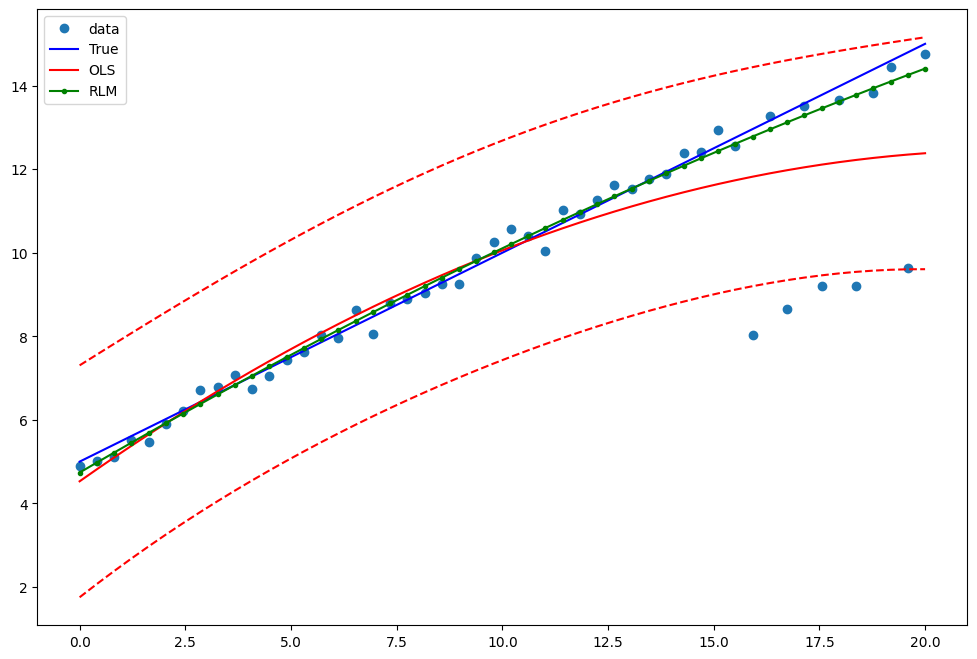
Example 1: quadratic function with linear truth
Note that the quadratic term in OLS regression will capture outlier effects.
[8]:
res = sm.OLS(y2, X).fit()
print(res.params)
print(res.bse)
print(res.predict())
[ 5.02820241  0.53204602 -0.01468896]
[0.44011628 0.06794801 0.00601235]
[ 4.66097829  4.93564775  5.20542292  5.47030381  5.73029042  5.98538275
  6.2355808   6.48088456  6.72129404  6.95680924  7.18743016  7.41315679
  7.63398914  7.84992721  8.060971    8.2671205   8.46837573  8.66473667
  8.85620333  9.0427757   9.22445379  9.40123761  9.57312713  9.74012238
  9.90222335 10.05943003 10.21174243 10.35916055 10.50168438 10.63931393
 10.7720492  10.89989019 11.0228369  11.14088932 11.25404746 11.36231132
 11.4656809  11.56415619 11.65773721 11.74642394 11.83021638 11.90911455
 11.98311843 12.05222803 12.11644335 12.17576439 12.23019114 12.27972361
 12.3243618  12.36410571]
Estimate RLM:
[9]:
resrlm = sm.RLM(y2, X).fit()
print(resrlm.params)
print(resrlm.bse)
[ 4.97638643e+00  5.14991250e-01 -4.20543868e-03]
[0.14961991 0.02309929 0.00204393]
Draw a plot to compare OLS estimates to the robust estimates:
[10]:
fig = plt.figure(figsize=(12, 8))
ax = fig.add_subplot(111)
ax.plot(x1, y2, "o", label="data")
ax.plot(x1, y_true2, "b-", label="True")
pred_ols = res.get_prediction()
iv_l = pred_ols.summary_frame()["obs_ci_lower"]
iv_u = pred_ols.summary_frame()["obs_ci_upper"]

ax.plot(x1, res.fittedvalues, "r-", label="OLS")
ax.plot(x1, iv_u, "r--")
ax.plot(x1, iv_l, "r--")
ax.plot(x1, resrlm.fittedvalues, "g.-", label="RLM")
ax.legend(loc="best")
[10]:
<matplotlib.legend.Legend at 0x7f490f656e00>
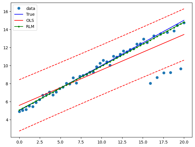
Example 2: linear function with linear truth
Fit a new OLS model using only the linear term and the constant:
[11]:
X2 = X[:, [0, 1]]
res2 = sm.OLS(y2, X2).fit()
print(res2.params)
print(res2.bse)
[5.62025762 0.38515637]
[0.38593896 0.03325406]
Estimate RLM:
[12]:
resrlm2 = sm.RLM(y2, X2).fit()
print(resrlm2.params)
print(resrlm2.bse)
[5.12579959 0.47660869]
[0.11586957 0.00998379]
Draw a plot to compare OLS estimates to the robust estimates:
[13]:
pred_ols = res2.get_prediction()
iv_l = pred_ols.summary_frame()["obs_ci_lower"]
iv_u = pred_ols.summary_frame()["obs_ci_upper"]

fig, ax = plt.subplots(figsize=(8, 6))
ax.plot(x1, y2, "o", label="data")
ax.plot(x1, y_true2, "b-", label="True")
ax.plot(x1, res2.fittedvalues, "r-", label="OLS")
ax.plot(x1, iv_u, "r--")
ax.plot(x1, iv_l, "r--")
ax.plot(x1, resrlm2.fittedvalues, "g.-", label="RLM")
legend = ax.legend(loc="best")
Last update:
May 14, 2024