Prediction (out of sample)
[1]:
%matplotlib inline
[2]:
import numpy as np
import statsmodels.api as sm
Artificial data
[3]:
nsample = 50
sig = 0.25
x1 = np.linspace(0, 20, nsample)
X = np.column_stack((x1, np.sin(x1), (x1-5)**2))
X = sm.add_constant(X)
beta = [5., 0.5, 0.5, -0.02]
y_true = np.dot(X, beta)
y = y_true + sig * np.random.normal(size=nsample)
Estimation
[4]:
olsmod = sm.OLS(y, X)
olsres = olsmod.fit()
print(olsres.summary())
                            OLS Regression Results
==============================================================================
Dep. Variable:                      y   R-squared:                       0.980
Model:                            OLS   Adj. R-squared:                  0.979
Method:                 Least Squares   F-statistic:                     754.1
Date:                Fri, 21 Feb 2020   Prob (F-statistic):           4.21e-39
Time:                        13:57:24   Log-Likelihood:                -4.1308
No. Observations:                  50   AIC:                             16.26
Df Residuals:                      46   BIC:                             23.91
Df Model:                           3
Covariance Type:            nonrobust
==============================================================================
                 coef    std err          t      P>|t|      [0.025      0.975]
------------------------------------------------------------------------------
const          5.0831      0.093     54.429      0.000       4.895       5.271
x1             0.4907      0.014     34.071      0.000       0.462       0.520
x2             0.5216      0.057      9.212      0.000       0.408       0.636
x3            -0.0189      0.001    -14.954      0.000      -0.021      -0.016
==============================================================================
Omnibus:                        2.536   Durbin-Watson:                   2.416
Prob(Omnibus):                  0.281   Jarque-Bera (JB):                1.892
Skew:                          -0.473   Prob(JB):                        0.388
Kurtosis:                       3.122   Cond. No.                         221.
==============================================================================

Warnings:
[1] Standard Errors assume that the covariance matrix of the errors is correctly specified.
In-sample prediction
[5]:
ypred = olsres.predict(X)
print(ypred)
[ 4.61036341  5.09172228  5.53276677  5.90507171  6.19047043  6.38403949
  6.49490757  6.54475568  6.56425502  6.58802778  6.64895881  6.77279276
  6.97390428  7.25293632  7.59669448  7.98031483  8.37134897  8.73509521
  9.04029999  9.2642927   9.39671042  9.44120056  9.41482152  9.3452401
  9.26618593  9.21190973  9.21155609  9.28437501  9.43655927  9.6602269
  9.93471621 10.22998043 10.5115243  10.74607157 10.90703217 10.97887089
 10.95965979 10.86139491 10.70802541 10.53151874 10.36660852 10.24508788
 10.19058594 10.21468562 10.31502061 10.47566411 10.6697456  10.86386558
 11.02358297 11.11907377]
Create a new sample of explanatory variables Xnew, predict and plot
[6]:
x1n = np.linspace(20.5,25, 10)
Xnew = np.column_stack((x1n, np.sin(x1n), (x1n-5)**2))
Xnew = sm.add_constant(Xnew)
ynewpred =  olsres.predict(Xnew) # predict out of sample
print(ynewpred)
[11.11980579 10.98378856 10.73147613 10.40948069 10.07916026  9.80159615
  9.62263807  9.56167858  9.60690506  9.71819191]
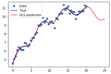
Plot comparison
[7]:
import matplotlib.pyplot as plt

fig, ax = plt.subplots()
ax.plot(x1, y, 'o', label="Data")
ax.plot(x1, y_true, 'b-', label="True")
ax.plot(np.hstack((x1, x1n)), np.hstack((ypred, ynewpred)), 'r', label="OLS prediction")
ax.legend(loc="best");
Predicting with Formulas
Using formulas can make both estimation and prediction a lot easier
[8]:
from statsmodels.formula.api import ols

data = {"x1" : x1, "y" : y}

res = ols("y ~ x1 + np.sin(x1) + I((x1-5)**2)", data=data).fit()
We use the I to indicate use of the Identity transform. Ie., we do not want any expansion magic from using **2
[9]:
res.params
[9]:
Intercept           5.083128
x1                  0.490733
np.sin(x1)          0.521571
I((x1 - 5) ** 2)   -0.018911
dtype: float64
Now we only have to pass the single variable and we get the transformed right-hand side variables automatically
[10]:
res.predict(exog=dict(x1=x1n))
[10]:
0    11.119806
1    10.983789
2    10.731476
3    10.409481
4    10.079160
5     9.801596
6     9.622638
7     9.561679
8     9.606905
9     9.718192
dtype: float64