VARMAX models
This is a brief introduction notebook to VARMAX models in statsmodels. The VARMAX model is generically specified as:
where \(y_t\) is a \(\text{k_endog} \times 1\) vector.
[1]:
%matplotlib inline
[2]:
import numpy as np
import pandas as pd
import statsmodels.api as sm
import matplotlib.pyplot as plt
[3]:
dta = sm.datasets.webuse('lutkepohl2', 'https://www.stata-press.com/data/r12/')
dta.index = dta.qtr
endog = dta.loc['1960-04-01':'1978-10-01', ['dln_inv', 'dln_inc', 'dln_consump']]
Model specification
The VARMAX class in statsmodels allows estimation of VAR, VMA, and VARMA models (through the order argument), optionally with a constant term (via the trend argument). Exogenous regressors may also be included (as usual in statsmodels, by the exog argument), and in this way a time trend may be added. Finally, the class allows measurement error (via the measurement_error argument) and allows specifying either a diagonal or unstructured innovation covariance matrix (via the
error_cov_type argument).
Example 1: VAR
Below is a simple VARX(2) model in two endogenous variables and an exogenous series, but no constant term. Notice that we needed to allow for more iterations than the default (which is maxiter=50) in order for the likelihood estimation to converge. This is not unusual in VAR models which have to estimate a large number of parameters, often on a relatively small number of time series: this model, for example, estimates 27 parameters off of 75 observations of 3 variables.
[4]:
exog = endog['dln_consump']
mod = sm.tsa.VARMAX(endog[['dln_inv', 'dln_inc']], order=(2,0), trend='n', exog=exog)
res = mod.fit(maxiter=1000, disp=False)
print(res.summary())
/home/travis/build/statsmodels/statsmodels/statsmodels/tsa/base/tsa_model.py:162: ValueWarning: No frequency information was provided, so inferred frequency QS-OCT will be used.
  % freq, ValueWarning)
                             Statespace Model Results
==================================================================================
Dep. Variable:     ['dln_inv', 'dln_inc']   No. Observations:                   75
Model:                            VARX(2)   Log Likelihood                 361.036
Date:                    Fri, 21 Feb 2020   AIC                           -696.072
Time:                            13:54:51   BIC                           -665.945
Sample:                        04-01-1960   HQIC                          -684.043
                             - 10-01-1978
Covariance Type:                      opg
===================================================================================
Ljung-Box (Q):                61.20, 39.27   Jarque-Bera (JB):          11.47, 2.34
Prob(Q):                        0.02, 0.50   Prob(JB):                   0.00, 0.31
Heteroskedasticity (H):         0.45, 0.40   Skew:                      0.16, -0.38
Prob(H) (two-sided):            0.05, 0.03   Kurtosis:                   4.89, 3.43
                            Results for equation dln_inv
====================================================================================
                       coef    std err          z      P>|z|      [0.025      0.975]
------------------------------------------------------------------------------------
L1.dln_inv          -0.2372      0.093     -2.544      0.011      -0.420      -0.054
L1.dln_inc           0.2837      0.449      0.632      0.528      -0.597       1.164
L2.dln_inv          -0.1648      0.156     -1.057      0.290      -0.470       0.141
L2.dln_inc           0.0754      0.422      0.178      0.858      -0.752       0.903
beta.dln_consump     0.9544      0.640      1.492      0.136      -0.300       2.208
                            Results for equation dln_inc
====================================================================================
                       coef    std err          z      P>|z|      [0.025      0.975]
------------------------------------------------------------------------------------
L1.dln_inv           0.0636      0.036      1.782      0.075      -0.006       0.134
L1.dln_inc           0.0847      0.107      0.793      0.428      -0.125       0.294
L2.dln_inv           0.0098      0.033      0.298      0.765      -0.055       0.074
L2.dln_inc           0.0356      0.134      0.265      0.791      -0.227       0.299
beta.dln_consump     0.7684      0.112      6.853      0.000       0.549       0.988
                                  Error covariance matrix
============================================================================================
                               coef    std err          z      P>|z|      [0.025      0.975]
--------------------------------------------------------------------------------------------
sqrt.var.dln_inv             0.0434      0.004     12.269      0.000       0.036       0.050
sqrt.cov.dln_inv.dln_inc  5.368e-05      0.002      0.027      0.979      -0.004       0.004
sqrt.var.dln_inc             0.0109      0.001     11.239      0.000       0.009       0.013
============================================================================================

Warnings:
[1] Covariance matrix calculated using the outer product of gradients (complex-step).
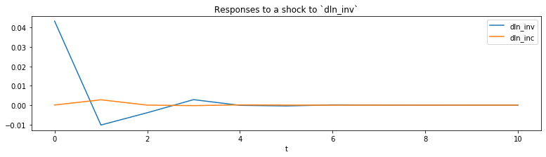
From the estimated VAR model, we can plot the impulse response functions of the endogenous variables.
[5]:
ax = res.impulse_responses(10, orthogonalized=True).plot(figsize=(13,3))
ax.set(xlabel='t', title='Responses to a shock to `dln_inv`');
Example 2: VMA
A vector moving average model can also be formulated. Below we show a VMA(2) on the same data, but where the innovations to the process are uncorrelated. In this example we leave out the exogenous regressor but now include the constant term.
[6]:
mod = sm.tsa.VARMAX(endog[['dln_inv', 'dln_inc']], order=(0,2), error_cov_type='diagonal')
res = mod.fit(maxiter=1000, disp=False)
print(res.summary())
/home/travis/build/statsmodels/statsmodels/statsmodels/tsa/base/tsa_model.py:162: ValueWarning: No frequency information was provided, so inferred frequency QS-OCT will be used.
  % freq, ValueWarning)
                             Statespace Model Results
==================================================================================
Dep. Variable:     ['dln_inv', 'dln_inc']   No. Observations:                   75
Model:                             VMA(2)   Log Likelihood                 353.887
                              + intercept   AIC                           -683.774
Date:                    Fri, 21 Feb 2020   BIC                           -655.964
Time:                            13:54:55   HQIC                          -672.670
Sample:                        04-01-1960
                             - 10-01-1978
Covariance Type:                      opg
===================================================================================
Ljung-Box (Q):                68.83, 39.18   Jarque-Bera (JB):         12.37, 13.43
Prob(Q):                        0.00, 0.51   Prob(JB):                   0.00, 0.00
Heteroskedasticity (H):         0.44, 0.81   Skew:                      0.05, -0.48
Prob(H) (two-sided):            0.04, 0.60   Kurtosis:                   4.99, 4.84
                           Results for equation dln_inv
=================================================================================
                    coef    std err          z      P>|z|      [0.025      0.975]
---------------------------------------------------------------------------------
intercept         0.0182      0.005      3.803      0.000       0.009       0.028
L1.e(dln_inv)    -0.2638      0.106     -2.499      0.012      -0.471      -0.057
L1.e(dln_inc)     0.5232      0.632      0.828      0.407      -0.715       1.761
L2.e(dln_inv)     0.0348      0.148      0.235      0.814      -0.255       0.324
L2.e(dln_inc)     0.1824      0.477      0.383      0.702      -0.752       1.117
                           Results for equation dln_inc
=================================================================================
                    coef    std err          z      P>|z|      [0.025      0.975]
---------------------------------------------------------------------------------
intercept         0.0207      0.002     13.029      0.000       0.018       0.024
L1.e(dln_inv)     0.0484      0.042      1.163      0.245      -0.033       0.130
L1.e(dln_inc)    -0.0755      0.139     -0.542      0.588      -0.349       0.198
L2.e(dln_inv)     0.0177      0.042      0.419      0.676      -0.065       0.101
L2.e(dln_inc)     0.1298      0.153      0.849      0.396      -0.170       0.429
                             Error covariance matrix
==================================================================================
                     coef    std err          z      P>|z|      [0.025      0.975]
----------------------------------------------------------------------------------
sigma2.dln_inv     0.0020      0.000      7.366      0.000       0.001       0.003
sigma2.dln_inc     0.0001   2.33e-05      5.818      0.000    8.99e-05       0.000
==================================================================================

Warnings:
[1] Covariance matrix calculated using the outer product of gradients (complex-step).
Caution: VARMA(p,q) specifications
Although the model allows estimating VARMA(p,q) specifications, these models are not identified without additional restrictions on the representation matrices, which are not built-in. For this reason, it is recommended that the user proceed with error (and indeed a warning is issued when these models are specified). Nonetheless, they may in some circumstances provide useful information.
[7]:
mod = sm.tsa.VARMAX(endog[['dln_inv', 'dln_inc']], order=(1,1))
res = mod.fit(maxiter=1000, disp=False)
print(res.summary())
/home/travis/build/statsmodels/statsmodels/statsmodels/tsa/statespace/varmax.py:163: EstimationWarning: Estimation of VARMA(p,q) models is not generically robust, due especially to identification issues.
  EstimationWarning)
/home/travis/build/statsmodels/statsmodels/statsmodels/tsa/base/tsa_model.py:162: ValueWarning: No frequency information was provided, so inferred frequency QS-OCT will be used.
  % freq, ValueWarning)
                             Statespace Model Results
==================================================================================
Dep. Variable:     ['dln_inv', 'dln_inc']   No. Observations:                   75
Model:                         VARMA(1,1)   Log Likelihood                 354.288
                              + intercept   AIC                           -682.576
Date:                    Fri, 21 Feb 2020   BIC                           -652.449
Time:                            13:54:57   HQIC                          -670.547
Sample:                        04-01-1960
                             - 10-01-1978
Covariance Type:                      opg
===================================================================================
Ljung-Box (Q):                68.33, 39.15   Jarque-Bera (JB):         11.07, 14.06
Prob(Q):                        0.00, 0.51   Prob(JB):                   0.00, 0.00
Heteroskedasticity (H):         0.43, 0.91   Skew:                      0.01, -0.46
Prob(H) (two-sided):            0.04, 0.81   Kurtosis:                   4.88, 4.92
                           Results for equation dln_inv
=================================================================================
                    coef    std err          z      P>|z|      [0.025      0.975]
---------------------------------------------------------------------------------
intercept         0.0105      0.066      0.160      0.873      -0.118       0.139
L1.dln_inv       -0.0061      0.699     -0.009      0.993      -1.375       1.363
L1.dln_inc        0.3822      2.763      0.138      0.890      -5.032       5.797
L1.e(dln_inv)    -0.2484      0.709     -0.350      0.726      -1.638       1.141
L1.e(dln_inc)     0.1247      3.012      0.041      0.967      -5.779       6.029
                           Results for equation dln_inc
=================================================================================
                    coef    std err          z      P>|z|      [0.025      0.975]
---------------------------------------------------------------------------------
intercept         0.0165      0.027      0.601      0.548      -0.037       0.070
L1.dln_inv       -0.0334      0.279     -0.119      0.905      -0.581       0.514
L1.dln_inc        0.2348      1.114      0.211      0.833      -1.950       2.419
L1.e(dln_inv)     0.0889      0.286      0.311      0.756      -0.471       0.649
L1.e(dln_inc)    -0.2382      1.149     -0.207      0.836      -2.490       2.014
                                  Error covariance matrix
============================================================================================
                               coef    std err          z      P>|z|      [0.025      0.975]
--------------------------------------------------------------------------------------------
sqrt.var.dln_inv             0.0449      0.003     14.523      0.000       0.039       0.051
sqrt.cov.dln_inv.dln_inc     0.0017      0.003      0.650      0.516      -0.003       0.007
sqrt.var.dln_inc             0.0116      0.001     11.712      0.000       0.010       0.013
============================================================================================

Warnings:
[1] Covariance matrix calculated using the outer product of gradients (complex-step).