Autoregressive Moving Average (ARMA): Sunspots data
[1]:
%matplotlib inline
[2]:
import numpy as np
from scipy import stats
import pandas as pd
import matplotlib.pyplot as plt

import statsmodels.api as sm
[3]:
from statsmodels.graphics.api import qqplot
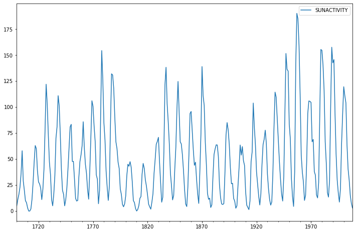
Sunspots Data
[4]:
print(sm.datasets.sunspots.NOTE)
::

    Number of Observations - 309 (Annual 1700 - 2008)
    Number of Variables - 1
    Variable name definitions::

        SUNACTIVITY - Number of sunspots for each year

    The data file contains a 'YEAR' variable that is not returned by load.
[5]:
dta = sm.datasets.sunspots.load_pandas().data
[6]:
dta.index = pd.Index(sm.tsa.datetools.dates_from_range('1700', '2008'))
del dta["YEAR"]
[7]:
dta.plot(figsize=(12,8));
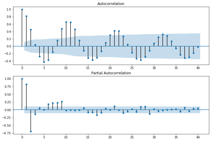
[8]:
fig = plt.figure(figsize=(12,8))
ax1 = fig.add_subplot(211)
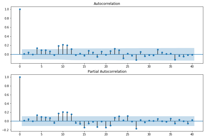
fig = sm.graphics.tsa.plot_acf(dta.values.squeeze(), lags=40, ax=ax1)
ax2 = fig.add_subplot(212)
fig = sm.graphics.tsa.plot_pacf(dta, lags=40, ax=ax2)
[9]:
arma_mod20 = sm.tsa.ARMA(dta, (2,0)).fit(disp=False)
print(arma_mod20.params)
const                49.659418
ar.L1.SUNACTIVITY     1.390656
ar.L2.SUNACTIVITY    -0.688571
dtype: float64
/home/travis/build/statsmodels/statsmodels/statsmodels/tsa/base/tsa_model.py:162: ValueWarning: No frequency information was provided, so inferred frequency A-DEC will be used.
  % freq, ValueWarning)
[10]:
arma_mod30 = sm.tsa.ARMA(dta, (3,0)).fit(disp=False)
/home/travis/build/statsmodels/statsmodels/statsmodels/tsa/base/tsa_model.py:162: ValueWarning: No frequency information was provided, so inferred frequency A-DEC will be used.
  % freq, ValueWarning)
[11]:
print(arma_mod20.aic, arma_mod20.bic, arma_mod20.hqic)
2622.6363380637504 2637.569703171341 2628.6067259089964
[12]:
print(arma_mod30.params)
const                49.749905
ar.L1.SUNACTIVITY     1.300810
ar.L2.SUNACTIVITY    -0.508093
ar.L3.SUNACTIVITY    -0.129649
dtype: float64
[13]:
print(arma_mod30.aic, arma_mod30.bic, arma_mod30.hqic)
2619.4036286966934 2638.0703350811823 2626.866613503251
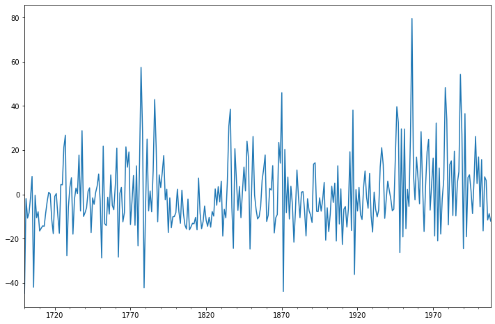
Does our model obey the theory?
[14]:
sm.stats.durbin_watson(arma_mod30.resid.values)
[14]:
1.9564806206172771
[15]:
fig = plt.figure(figsize=(12,8))
ax = fig.add_subplot(111)
ax = arma_mod30.resid.plot(ax=ax);
[16]:
resid = arma_mod30.resid
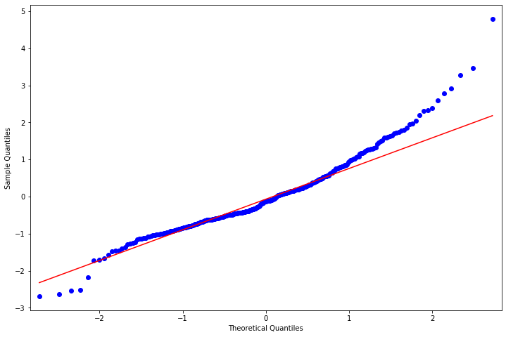
[17]:
stats.normaltest(resid)
[17]:
NormaltestResult(statistic=49.84504478123703, pvalue=1.5006729372147695e-11)
[18]:
fig = plt.figure(figsize=(12,8))
ax = fig.add_subplot(111)
fig = qqplot(resid, line='q', ax=ax, fit=True)
[19]:
fig = plt.figure(figsize=(12,8))
ax1 = fig.add_subplot(211)
fig = sm.graphics.tsa.plot_acf(resid.values.squeeze(), lags=40, ax=ax1)
ax2 = fig.add_subplot(212)
fig = sm.graphics.tsa.plot_pacf(resid, lags=40, ax=ax2)
[20]:
r,q,p = sm.tsa.acf(resid.values.squeeze(), fft=True, qstat=True)
data = np.c_[range(1,41), r[1:], q, p]
table = pd.DataFrame(data, columns=['lag', "AC", "Q", "Prob(>Q)"])
print(table.set_index('lag'))
            AC          Q      Prob(>Q)
lag
1.0   0.009179   0.026287  8.712011e-01
2.0   0.041794   0.573049  7.508687e-01
3.0  -0.001335   0.573608  9.024467e-01
4.0   0.136089   6.408928  1.706198e-01
5.0   0.092468   9.111833  1.046858e-01
6.0   0.091948  11.793244  6.674345e-02
7.0   0.068748  13.297202  6.518981e-02
8.0  -0.015020  13.369229  9.976133e-02
9.0   0.187592  24.641919  3.393898e-03
10.0  0.213718  39.322016  2.229455e-05
11.0  0.201082  52.361172  2.344915e-07
12.0  0.117182  56.804233  8.574099e-08
13.0 -0.014055  56.868369  1.893868e-07
14.0  0.015398  56.945609  3.997587e-07
15.0 -0.024967  57.149364  7.741333e-07
16.0  0.080916  59.296810  6.872056e-07
17.0  0.041138  59.853777  1.110927e-06
18.0 -0.052021  60.747467  1.548409e-06
19.0  0.062496  62.041732  1.831616e-06
20.0 -0.010301  62.077019  3.381194e-06
21.0  0.074453  63.926697  3.193536e-06
22.0  0.124955  69.154818  8.978200e-07
23.0  0.093162  72.071085  5.799677e-07
24.0 -0.082152  74.346735  4.712934e-07
25.0  0.015695  74.430091  8.288901e-07
26.0 -0.025037  74.642950  1.367261e-06
27.0 -0.125861  80.041200  3.722497e-07
28.0  0.053225  81.010031  4.716196e-07
29.0 -0.038693  81.523858  6.916510e-07
30.0 -0.016904  81.622277  1.151641e-06
31.0 -0.019296  81.750988  1.868734e-06
32.0  0.104990  85.575117  8.927801e-07
33.0  0.040086  86.134619  1.247487e-06
34.0  0.008829  86.161863  2.047790e-06
35.0  0.014588  86.236500  3.263752e-06
36.0 -0.119329  91.248951  1.084435e-06
37.0 -0.036666  91.723920  1.521896e-06
38.0 -0.046193  92.480571  1.938700e-06
39.0 -0.017768  92.592941  2.990625e-06
40.0 -0.006220  92.606764  4.696901e-06
This indicates a lack of fit.
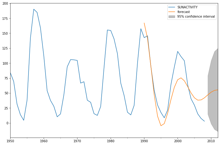
In-sample dynamic prediction. How good does our model do?
[21]:
predict_sunspots = arma_mod30.predict('1990', '2012', dynamic=True)
print(predict_sunspots)
1990-12-31    167.047383
1991-12-31    140.992929
1992-12-31     94.859019
1993-12-31     46.860813
1994-12-31     11.242529
1995-12-31     -4.721307
1996-12-31     -1.166890
1997-12-31     16.185729
1998-12-31     39.021913
1999-12-31     59.449874
2000-12-31     72.170109
2001-12-31     75.376718
2002-12-31     70.436375
2003-12-31     60.731501
2004-12-31     50.201726
2005-12-31     42.075980
2006-12-31     38.114265
2007-12-31     38.454638
2008-12-31     41.963816
2009-12-31     46.869281
2010-12-31     51.423242
2011-12-31     54.399683
2012-12-31     55.321642
Freq: A-DEC, dtype: float64
[22]:
fig, ax = plt.subplots(figsize=(12, 8))
ax = dta.loc['1950':].plot(ax=ax)
fig = arma_mod30.plot_predict('1990', '2012', dynamic=True, ax=ax, plot_insample=False)
[23]:
def mean_forecast_err(y, yhat):
    return y.sub(yhat).mean()
[24]:
mean_forecast_err(dta.SUNACTIVITY, predict_sunspots)
[24]:
5.636993629037569
Exercise: Can you obtain a better fit for the Sunspots model? (Hint: sm.tsa.AR has a method select_order)
Simulated ARMA(4,1): Model Identification is Difficult
[25]:
from statsmodels.tsa.arima_process import ArmaProcess
[26]:
np.random.seed(1234)
# include zero-th lag
arparams = np.array([1, .75, -.65, -.55, .9])
maparams = np.array([1, .65])
Let’s make sure this model is estimable.
[27]:
arma_t = ArmaProcess(arparams, maparams)
[28]:
arma_t.isinvertible
[28]:
True
[29]:
arma_t.isstationary
[29]:
False
What does this mean?
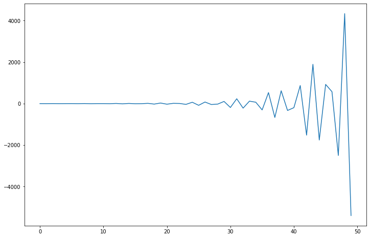
[30]:
fig = plt.figure(figsize=(12,8))
ax = fig.add_subplot(111)
ax.plot(arma_t.generate_sample(nsample=50));
[31]:
arparams = np.array([1, .35, -.15, .55, .1])
maparams = np.array([1, .65])
arma_t = ArmaProcess(arparams, maparams)
arma_t.isstationary
[31]:
True
[32]:
arma_rvs = arma_t.generate_sample(nsample=500, burnin=250, scale=2.5)
[33]:
fig = plt.figure(figsize=(12,8))
ax1 = fig.add_subplot(211)
fig = sm.graphics.tsa.plot_acf(arma_rvs, lags=40, ax=ax1)
ax2 = fig.add_subplot(212)
fig = sm.graphics.tsa.plot_pacf(arma_rvs, lags=40, ax=ax2)
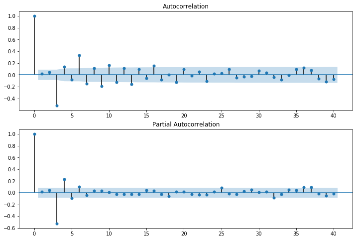
For mixed ARMA processes the Autocorrelation function is a mixture of exponentials and damped sine waves after (q-p) lags.
The partial autocorrelation function is a mixture of exponentials and dampened sine waves after (p-q) lags.
[34]:
arma11 = sm.tsa.ARMA(arma_rvs, (1,1)).fit(disp=False)
resid = arma11.resid
r,q,p = sm.tsa.acf(resid, fft=True, qstat=True)
data = np.c_[range(1,41), r[1:], q, p]
table = pd.DataFrame(data, columns=['lag', "AC", "Q", "Prob(>Q)"])
print(table.set_index('lag'))
            AC           Q      Prob(>Q)
lag
1.0   0.254921   32.687679  1.082211e-08
2.0  -0.172416   47.670749  4.450700e-11
3.0  -0.420945  137.159394  1.548465e-29
4.0  -0.046875  138.271303  6.617697e-29
5.0   0.103240  143.675911  2.958716e-29
6.0   0.214864  167.133000  1.823717e-33
7.0  -0.000889  167.133402  1.009205e-32
8.0  -0.045418  168.185755  3.094832e-32
9.0  -0.061445  170.115804  5.837211e-32
10.0  0.034623  170.729856  1.958736e-31
11.0  0.006351  170.750557  8.267050e-31
12.0 -0.012882  170.835910  3.220231e-30
13.0 -0.053959  172.336547  6.181196e-30
14.0 -0.016606  172.478965  2.160215e-29
15.0  0.051742  173.864489  4.089542e-29
16.0  0.078917  177.094280  3.217937e-29
17.0 -0.001834  177.096028  1.093168e-28
18.0 -0.101604  182.471939  3.103820e-29
19.0 -0.057342  184.187772  4.624066e-29
20.0  0.026975  184.568285  1.235671e-28
21.0  0.062359  186.605964  1.530258e-28
22.0 -0.009400  186.652366  4.548192e-28
23.0 -0.068037  189.088184  4.562012e-28
24.0 -0.035566  189.755202  9.901092e-28
25.0  0.095679  194.592626  3.354283e-28
26.0  0.065650  196.874879  3.487619e-28
27.0 -0.018404  197.054614  9.008743e-28
28.0 -0.079244  200.394013  5.773702e-28
29.0  0.008499  200.432506  1.541383e-27
30.0  0.053372  201.953778  2.133189e-27
31.0  0.074816  204.949400  1.550158e-27
32.0 -0.071187  207.667250  1.262284e-27
33.0 -0.088145  211.843160  5.480804e-28
34.0 -0.025283  212.187455  1.215225e-27
35.0  0.125690  220.714908  8.231574e-29
36.0  0.142724  231.734123  1.923077e-30
37.0  0.095768  236.706168  5.937760e-31
38.0 -0.084744  240.607813  2.890873e-31
39.0 -0.150126  252.878989  3.962990e-33
40.0 -0.083767  256.707748  1.996165e-33
[35]:
arma41 = sm.tsa.ARMA(arma_rvs, (4,1)).fit(disp=False)
resid = arma41.resid
r,q,p = sm.tsa.acf(resid, fft=True, qstat=True)
data = np.c_[range(1,41), r[1:], q, p]
table = pd.DataFrame(data, columns=['lag', "AC", "Q", "Prob(>Q)"])
print(table.set_index('lag'))
            AC          Q  Prob(>Q)
lag
1.0  -0.007888   0.031301  0.859571
2.0   0.004132   0.039906  0.980245
3.0   0.018103   0.205416  0.976710
4.0  -0.006760   0.228539  0.993948
5.0   0.018120   0.395025  0.995466
6.0   0.050688   1.700447  0.945087
7.0   0.010252   1.753954  0.972197
8.0  -0.011206   1.818017  0.986092
9.0   0.020292   2.028517  0.991009
10.0  0.001029   2.029059  0.996113
11.0 -0.014035   2.130167  0.997984
12.0 -0.023858   2.422925  0.998427
13.0 -0.002108   2.425215  0.999339
14.0 -0.018783   2.607428  0.999590
15.0  0.011316   2.673698  0.999805
16.0  0.042159   3.595418  0.999443
17.0  0.007943   3.628204  0.999734
18.0 -0.074311   6.503854  0.993686
19.0 -0.023379   6.789066  0.995256
20.0  0.002398   6.792072  0.997313
21.0  0.000487   6.792197  0.998516
22.0  0.017952   6.961434  0.999024
23.0 -0.038576   7.744465  0.998744
24.0 -0.029816   8.213248  0.998859
25.0  0.077850  11.415823  0.990675
26.0  0.040408  12.280447  0.989479
27.0 -0.018612  12.464274  0.992262
28.0 -0.014764  12.580185  0.994586
29.0  0.017650  12.746189  0.996111
30.0 -0.005486  12.762262  0.997504
31.0  0.058256  14.578543  0.994614
32.0 -0.040840  15.473082  0.993887
33.0 -0.019493  15.677307  0.995393
34.0  0.037269  16.425464  0.995214
35.0  0.086212  20.437447  0.976296
36.0  0.041271  21.358845  0.974774
37.0  0.078704  24.716877  0.938948
38.0 -0.029729  25.197054  0.944895
39.0 -0.078397  28.543385  0.891179
40.0 -0.014466  28.657576  0.909268
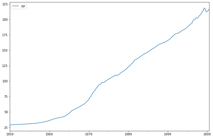
Exercise: How good of in-sample prediction can you do for another series, say, CPI
[36]:
macrodta = sm.datasets.macrodata.load_pandas().data
macrodta.index = pd.Index(sm.tsa.datetools.dates_from_range('1959Q1', '2009Q3'))
cpi = macrodta["cpi"]
Hint:
[37]:
fig = plt.figure(figsize=(12,8))
ax = fig.add_subplot(111)
ax = cpi.plot(ax=ax);
ax.legend();
P-value of the unit-root test, resoundingly rejects the null of a unit-root.
[38]:
print(sm.tsa.adfuller(cpi)[1])
0.9904328188337421