Prediction (out of sample)
[1]:
%matplotlib inline
[2]:
import numpy as np
import matplotlib.pyplot as plt

import statsmodels.api as sm

plt.rc("figure", figsize=(16, 8))
plt.rc("font", size=14)
Artificial data
[3]:
nsample = 50
sig = 0.25
x1 = np.linspace(0, 20, nsample)
X = np.column_stack((x1, np.sin(x1), (x1 - 5) ** 2))
X = sm.add_constant(X)
beta = [5.0, 0.5, 0.5, -0.02]
y_true = np.dot(X, beta)
y = y_true + sig * np.random.normal(size=nsample)
Estimation
[4]:
olsmod = sm.OLS(y, X)
olsres = olsmod.fit()
print(olsres.summary())
                            OLS Regression Results
==============================================================================
Dep. Variable:                      y   R-squared:                       0.985
Model:                            OLS   Adj. R-squared:                  0.984
Method:                 Least Squares   F-statistic:                     992.2
Date:                Fri, 05 Dec 2025   Prob (F-statistic):           8.55e-42
Time:                        18:07:35   Log-Likelihood:                 3.2615
No. Observations:                  50   AIC:                             1.477
Df Residuals:                      46   BIC:                             9.125
Df Model:                           3
Covariance Type:            nonrobust
==============================================================================
                 coef    std err          t      P>|t|      [0.025      0.975]
------------------------------------------------------------------------------
const          5.1446      0.081     63.865      0.000       4.982       5.307
x1             0.4839      0.012     38.950      0.000       0.459       0.509
x2             0.5656      0.049     11.582      0.000       0.467       0.664
x3            -0.0185      0.001    -16.996      0.000      -0.021      -0.016
==============================================================================
Omnibus:                       12.733   Durbin-Watson:                   2.397
Prob(Omnibus):                  0.002   Jarque-Bera (JB):               14.058
Skew:                           0.993   Prob(JB):                     0.000886
Kurtosis:                       4.674   Cond. No.                         221.
==============================================================================

Notes:
[1] Standard Errors assume that the covariance matrix of the errors is correctly specified.
In-sample prediction
[5]:
ypred = olsres.predict(X)
print(ypred)
[ 4.68113833  5.17574257  5.62728302  6.00493338  6.28899241  6.47412076
  6.57021825  6.60079732  6.59912001  6.60273313  6.64729937  6.7607381
  6.9586382   7.24169694  7.59560537  7.99339925  8.39988919  8.77744221
  9.09216466  9.31947092  9.44812271  9.48207552  9.43982871  9.35138616
  9.2533267   9.18279428  9.17139537  9.24000609  9.39534231  9.62885627
  9.91814093 10.23061142 10.5288586  10.77679531 10.94558536 11.01838126
 10.9930922  10.88272756 10.71325952 10.5193559  10.33868432 10.20572354
 10.14609869 10.17237113 10.28197463 10.45763704 10.67021804 10.8834968
 11.06012295 11.16775317]
Create a new sample of explanatory variables Xnew, predict and plot
[6]:
x1n = np.linspace(20.5, 25, 10)
Xnew = np.column_stack((x1n, np.sin(x1n), (x1n - 5) ** 2))
Xnew = sm.add_constant(Xnew)
ynewpred = olsres.predict(Xnew)  # predict out of sample
print(ynewpred)
[11.17443065 11.03379185 10.76801862 10.42766054 10.0792587   9.78905405
  9.60676932  9.55343519  9.61624123  9.75167231]
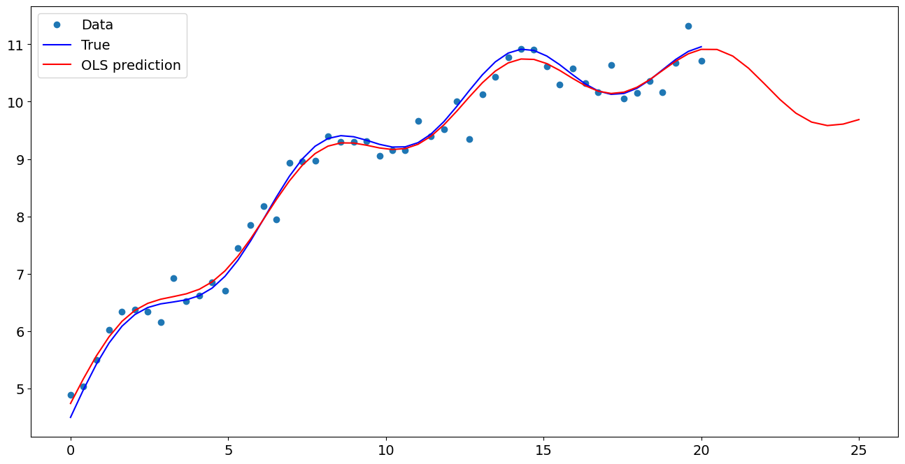
Plot comparison
[7]:
import matplotlib.pyplot as plt

fig, ax = plt.subplots()
ax.plot(x1, y, "o", label="Data")
ax.plot(x1, y_true, "b-", label="True")
ax.plot(np.hstack((x1, x1n)), np.hstack((ypred, ynewpred)), "r", label="OLS prediction")
ax.legend(loc="best")
[7]:
<matplotlib.legend.Legend at 0x7f9813dff490>
Predicting with Formulas
Using formulas can make both estimation and prediction a lot easier
[8]:
from statsmodels.formula.api import ols

data = {"x1": x1, "y": y}

res = ols("y ~ x1 + np.sin(x1) + I((x1-5)**2)", data=data).fit()
We use the I to indicate use of the Identity transform. Ie., we do not want any expansion magic from using **2
[9]:
res.params
[9]:
Intercept           5.144616
x1                  0.483902
np.sin(x1)          0.565629
I((x1 - 5) ** 2)   -0.018539
dtype: float64
Now we only have to pass the single variable and we get the transformed right-hand side variables automatically
[10]:
res.predict(exog=dict(x1=x1n))
[10]:
0    11.174431
1    11.033792
2    10.768019
3    10.427661
4    10.079259
5     9.789054
6     9.606769
7     9.553435
8     9.616241
9     9.751672
dtype: float64