Generalized Linear Models
[1]:
%matplotlib inline
[2]:
import numpy as np
import statsmodels.api as sm
from scipy import stats
from matplotlib import pyplot as plt

plt.rc("figure", figsize=(16,8))
plt.rc("font", size=14)
GLM: Binomial response data
Load Star98 data
In this example, we use the Star98 dataset which was taken with permission from Jeff Gill (2000) Generalized linear models: A unified approach. Codebook information can be obtained by typing:
[3]:
print(sm.datasets.star98.NOTE)
::

    Number of Observations - 303 (counties in California).

    Number of Variables - 13 and 8 interaction terms.

    Definition of variables names::

        NABOVE   - Total number of students above the national median for the
                   math section.
        NBELOW   - Total number of students below the national median for the
                   math section.
        LOWINC   - Percentage of low income students
        PERASIAN - Percentage of Asian student
        PERBLACK - Percentage of black students
        PERHISP  - Percentage of Hispanic students
        PERMINTE - Percentage of minority teachers
        AVYRSEXP - Sum of teachers' years in educational service divided by the
                number of teachers.
        AVSALK   - Total salary budget including benefits divided by the number
                   of full-time teachers (in thousands)
        PERSPENK - Per-pupil spending (in thousands)
        PTRATIO  - Pupil-teacher ratio.
        PCTAF    - Percentage of students taking UC/CSU prep courses
        PCTCHRT  - Percentage of charter schools
        PCTYRRND - Percentage of year-round schools

        The below variables are interaction terms of the variables defined
        above.

        PERMINTE_AVYRSEXP
        PEMINTE_AVSAL
        AVYRSEXP_AVSAL
        PERSPEN_PTRATIO
        PERSPEN_PCTAF
        PTRATIO_PCTAF
        PERMINTE_AVTRSEXP_AVSAL
        PERSPEN_PTRATIO_PCTAF
Load the data and add a constant to the exogenous (independent) variables:
[4]:
data = sm.datasets.star98.load(as_pandas=False)
data.exog = sm.add_constant(data.exog, prepend=False)
The dependent variable is N by 2 (Success: NABOVE, Failure: NBELOW):
[5]:
print(data.endog[:5,:])
[[452. 355.]
 [144.  40.]
 [337. 234.]
 [395. 178.]
 [  8.  57.]]
The independent variables include all the other variables described above, as well as the interaction terms:
[6]:
print(data.exog[:2,:])
[[3.43973000e+01 2.32993000e+01 1.42352800e+01 1.14111200e+01
  1.59183700e+01 1.47064600e+01 5.91573200e+01 4.44520700e+00
  2.17102500e+01 5.70327600e+01 0.00000000e+00 2.22222200e+01
  2.34102872e+02 9.41688110e+02 8.69994800e+02 9.65065600e+01
  2.53522420e+02 1.23819550e+03 1.38488985e+04 5.50403520e+03
  1.00000000e+00]
 [1.73650700e+01 2.93283800e+01 8.23489700e+00 9.31488400e+00
  1.36363600e+01 1.60832400e+01 5.95039700e+01 5.26759800e+00
  2.04427800e+01 6.46226400e+01 0.00000000e+00 0.00000000e+00
  2.19316851e+02 8.11417560e+02 9.57016600e+02 1.07684350e+02
  3.40406090e+02 1.32106640e+03 1.30502233e+04 6.95884680e+03
  1.00000000e+00]]
Fit and summary
[7]:
glm_binom = sm.GLM(data.endog, data.exog, family=sm.families.Binomial())
res = glm_binom.fit()
print(res.summary())
                 Generalized Linear Model Regression Results
==============================================================================
Dep. Variable:           ['y1', 'y2']   No. Observations:                  303
Model:                            GLM   Df Residuals:                      282
Model Family:                Binomial   Df Model:                           20
Link Function:                  logit   Scale:                          1.0000
Method:                          IRLS   Log-Likelihood:                -2998.6
Date:                Tue, 02 Feb 2021   Deviance:                       4078.8
Time:                        06:54:02   Pearson chi2:                 4.05e+03
No. Iterations:                     5
Covariance Type:            nonrobust
==============================================================================
                 coef    std err          z      P>|z|      [0.025      0.975]
------------------------------------------------------------------------------
x1            -0.0168      0.000    -38.749      0.000      -0.018      -0.016
x2             0.0099      0.001     16.505      0.000       0.009       0.011
x3            -0.0187      0.001    -25.182      0.000      -0.020      -0.017
x4            -0.0142      0.000    -32.818      0.000      -0.015      -0.013
x5             0.2545      0.030      8.498      0.000       0.196       0.313
x6             0.2407      0.057      4.212      0.000       0.129       0.353
x7             0.0804      0.014      5.775      0.000       0.053       0.108
x8            -1.9522      0.317     -6.162      0.000      -2.573      -1.331
x9            -0.3341      0.061     -5.453      0.000      -0.454      -0.214
x10           -0.1690      0.033     -5.169      0.000      -0.233      -0.105
x11            0.0049      0.001      3.921      0.000       0.002       0.007
x12           -0.0036      0.000    -15.878      0.000      -0.004      -0.003
x13           -0.0141      0.002     -7.391      0.000      -0.018      -0.010
x14           -0.0040      0.000     -8.450      0.000      -0.005      -0.003
x15           -0.0039      0.001     -4.059      0.000      -0.006      -0.002
x16            0.0917      0.015      6.321      0.000       0.063       0.120
x17            0.0490      0.007      6.574      0.000       0.034       0.064
x18            0.0080      0.001      5.362      0.000       0.005       0.011
x19            0.0002   2.99e-05      7.428      0.000       0.000       0.000
x20           -0.0022      0.000     -6.445      0.000      -0.003      -0.002
const          2.9589      1.547      1.913      0.056      -0.073       5.990
==============================================================================
Quantities of interest
[8]:
print('Total number of trials:',  data.endog[0].sum())
print('Parameters: ', res.params)
print('T-values: ', res.tvalues)
Total number of trials: 807.0
Parameters:  [-1.68150366e-02  9.92547661e-03 -1.87242148e-02 -1.42385609e-02
  2.54487173e-01  2.40693664e-01  8.04086739e-02 -1.95216050e+00
 -3.34086475e-01 -1.69022168e-01  4.91670212e-03 -3.57996435e-03
 -1.40765648e-02 -4.00499176e-03 -3.90639579e-03  9.17143006e-02
  4.89898381e-02  8.04073890e-03  2.22009503e-04 -2.24924861e-03
  2.95887793e+00]
T-values:  [-38.74908321  16.50473627 -25.1821894  -32.81791308   8.49827113
   4.21247925   5.7749976   -6.16191078  -5.45321673  -5.16865445
   3.92119964 -15.87825999  -7.39093058  -8.44963886  -4.05916246
   6.3210987    6.57434662   5.36229044   7.42806363  -6.44513698
   1.91301155]
First differences: We hold all explanatory variables constant at their means and manipulate the percentage of low income households to assess its impact on the response variables:
[9]:
means = data.exog.mean(axis=0)
means25 = means.copy()
means25[0] = stats.scoreatpercentile(data.exog[:,0], 25)
means75 = means.copy()
means75[0] = lowinc_75per = stats.scoreatpercentile(data.exog[:,0], 75)
resp_25 = res.predict(means25)
resp_75 = res.predict(means75)
diff = resp_75 - resp_25
The interquartile first difference for the percentage of low income households in a school district is:
[10]:
print("%2.4f%%" % (diff*100))
-11.8753%
Plots
We extract information that will be used to draw some interesting plots:
[11]:
nobs = res.nobs
y = data.endog[:,0]/data.endog.sum(1)
yhat = res.mu
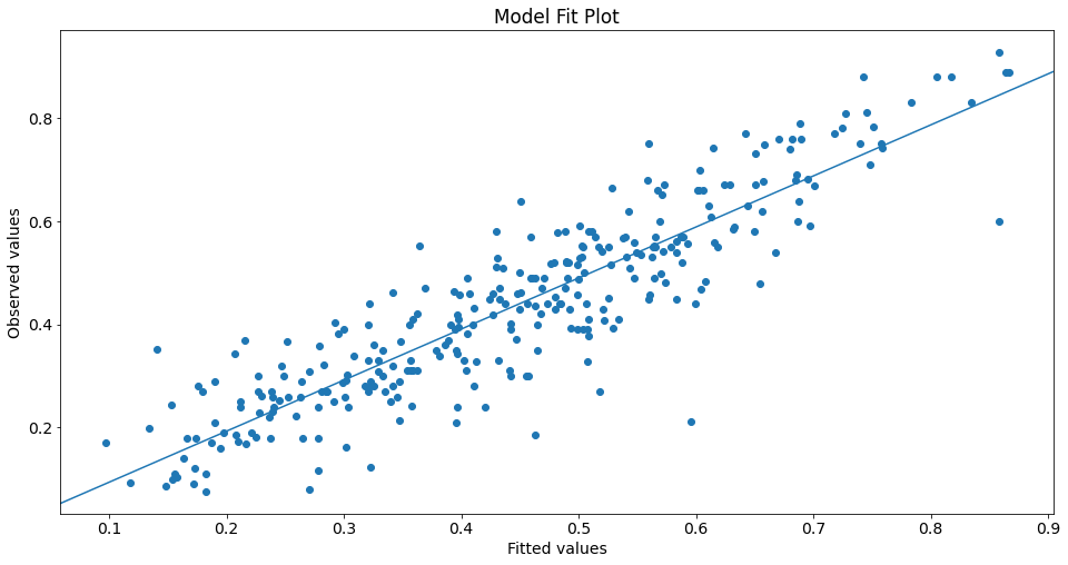
Plot yhat vs y:
[12]:
from statsmodels.graphics.api import abline_plot
[13]:
fig, ax = plt.subplots()
ax.scatter(yhat, y)
line_fit = sm.OLS(y, sm.add_constant(yhat, prepend=True)).fit()
abline_plot(model_results=line_fit, ax=ax)


ax.set_title('Model Fit Plot')
ax.set_ylabel('Observed values')
ax.set_xlabel('Fitted values');
[13]:
Text(0.5, 0, 'Fitted values')

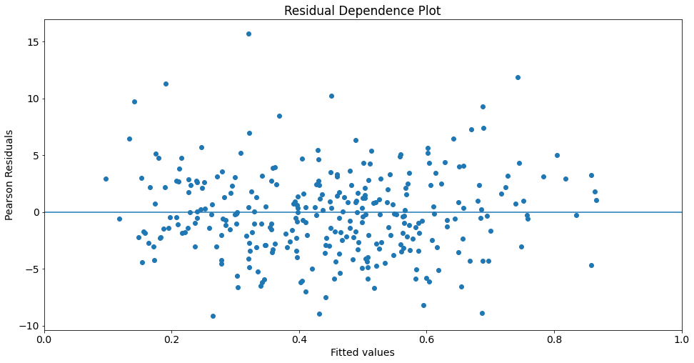
Plot yhat vs. Pearson residuals:
[14]:
fig, ax = plt.subplots()

ax.scatter(yhat, res.resid_pearson)
ax.hlines(0, 0, 1)
ax.set_xlim(0, 1)
ax.set_title('Residual Dependence Plot')
ax.set_ylabel('Pearson Residuals')
ax.set_xlabel('Fitted values')
[14]:
Text(0.5, 0, 'Fitted values')

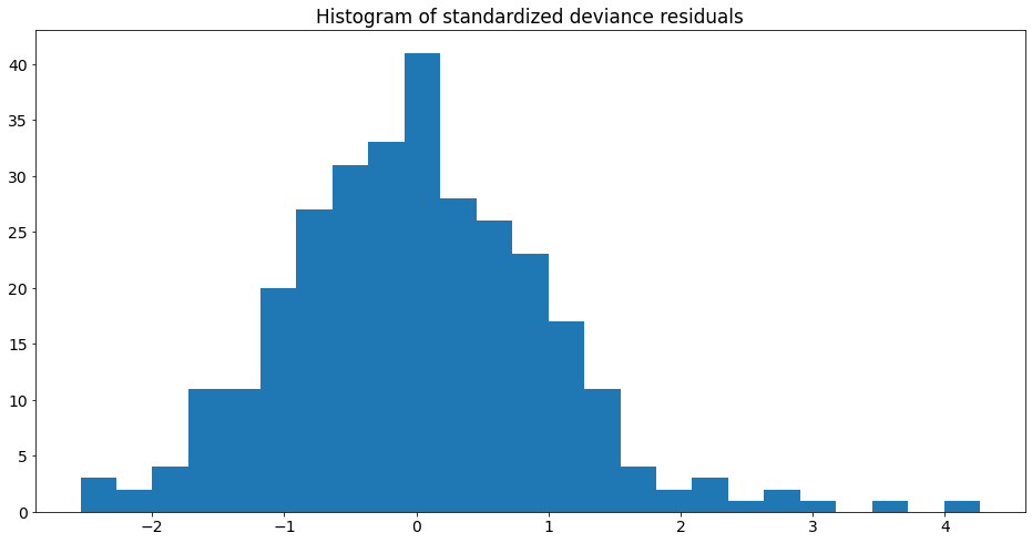
Histogram of standardized deviance residuals:
[15]:
from scipy import stats

fig, ax = plt.subplots()

resid = res.resid_deviance.copy()
resid_std = stats.zscore(resid)
ax.hist(resid_std, bins=25)
ax.set_title('Histogram of standardized deviance residuals');
[15]:
Text(0.5, 1.0, 'Histogram of standardized deviance residuals')

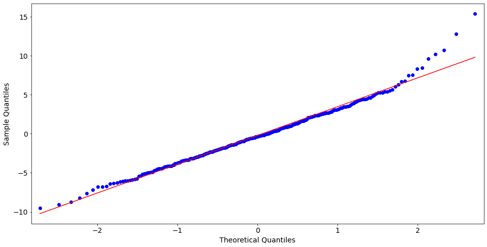
QQ Plot of Deviance Residuals:
[16]:
from statsmodels import graphics
graphics.gofplots.qqplot(resid, line='r')
[16]:


GLM: Gamma for proportional count response
Load Scottish Parliament Voting data
In the example above, we printed the NOTE attribute to learn about the Star98 dataset. statsmodels datasets ships with other useful information. For example:
[17]:
print(sm.datasets.scotland.DESCRLONG)
This data is based on the example in Gill and describes the proportion of
voters who voted Yes to grant the Scottish Parliament taxation powers.
The data are divided into 32 council districts.  This example's explanatory
variables include the amount of council tax collected in pounds sterling as
of April 1997 per two adults before adjustments, the female percentage of
total claims for unemployment benefits as of January, 1998, the standardized
mortality rate (UK is 100), the percentage of labor force participation,
regional GDP, the percentage of children aged 5 to 15, and an interaction term
between female unemployment and the council tax.

The original source files and variable information are included in
/scotland/src/
Load the data and add a constant to the exogenous variables:
[18]:
data2 = sm.datasets.scotland.load()
data2.exog = sm.add_constant(data2.exog, prepend=False)
print(data2.exog[:5,:])
print(data2.endog[:5])
[[7.12000e+02 2.10000e+01 1.05000e+02 8.24000e+01 1.35660e+04 1.23000e+01
  1.49520e+04 1.00000e+00]
 [6.43000e+02 2.65000e+01 9.70000e+01 8.02000e+01 1.35660e+04 1.53000e+01
  1.70395e+04 1.00000e+00]
 [6.79000e+02 2.83000e+01 1.13000e+02 8.63000e+01 9.61100e+03 1.39000e+01
  1.92157e+04 1.00000e+00]
 [8.01000e+02 2.71000e+01 1.09000e+02 8.04000e+01 9.48300e+03 1.36000e+01
  2.17071e+04 1.00000e+00]
 [7.53000e+02 2.20000e+01 1.15000e+02 6.47000e+01 9.26500e+03 1.46000e+01
  1.65660e+04 1.00000e+00]]
[60.3 52.3 53.4 57.  68.7]
Model Fit and summary
[19]:
glm_gamma = sm.GLM(data2.endog, data2.exog, family=sm.families.Gamma(sm.families.links.log()))
glm_results = glm_gamma.fit()
print(glm_results.summary())
                 Generalized Linear Model Regression Results
==============================================================================
Dep. Variable:                      y   No. Observations:                   32
Model:                            GLM   Df Residuals:                       24
Model Family:                   Gamma   Df Model:                            7
Link Function:                    log   Scale:                       0.0035927
Method:                          IRLS   Log-Likelihood:                -83.110
Date:                Tue, 02 Feb 2021   Deviance:                     0.087988
Time:                        06:54:04   Pearson chi2:                   0.0862
No. Iterations:                     7
Covariance Type:            nonrobust
==============================================================================
                 coef    std err          z      P>|z|      [0.025      0.975]
------------------------------------------------------------------------------
x1            -0.0024      0.001     -2.466      0.014      -0.004      -0.000
x2            -0.1005      0.031     -3.269      0.001      -0.161      -0.040
x3             0.0048      0.002      2.946      0.003       0.002       0.008
x4            -0.0067      0.003     -2.534      0.011      -0.012      -0.002
x5          8.173e-06   7.19e-06      1.136      0.256   -5.93e-06    2.23e-05
x6             0.0298      0.015      2.009      0.045       0.001       0.059
x7             0.0001   4.33e-05      2.724      0.006    3.31e-05       0.000
const          5.6581      0.680      8.318      0.000       4.325       6.991
==============================================================================
GLM: Gaussian distribution with a noncanonical link
Artificial data
[20]:
nobs2 = 100
x = np.arange(nobs2)
np.random.seed(54321)
X = np.column_stack((x,x**2))
X = sm.add_constant(X, prepend=False)
lny = np.exp(-(.03*x + .0001*x**2 - 1.0)) + .001 * np.random.rand(nobs2)
Fit and summary (artificial data)
[21]:
gauss_log = sm.GLM(lny, X, family=sm.families.Gaussian(sm.families.links.log()))
gauss_log_results = gauss_log.fit()
print(gauss_log_results.summary())
                 Generalized Linear Model Regression Results
==============================================================================
Dep. Variable:                      y   No. Observations:                  100
Model:                            GLM   Df Residuals:                       97
Model Family:                Gaussian   Df Model:                            2
Link Function:                    log   Scale:                      1.0531e-07
Method:                          IRLS   Log-Likelihood:                 662.92
Date:                Tue, 02 Feb 2021   Deviance:                   1.0215e-05
Time:                        06:54:04   Pearson chi2:                 1.02e-05
No. Iterations:                     7
Covariance Type:            nonrobust
==============================================================================
                 coef    std err          z      P>|z|      [0.025      0.975]
------------------------------------------------------------------------------
x1            -0.0300    5.6e-06  -5361.316      0.000      -0.030      -0.030
x2         -9.939e-05   1.05e-07   -951.091      0.000   -9.96e-05   -9.92e-05
const          1.0003   5.39e-05   1.86e+04      0.000       1.000       1.000
==============================================================================