statsmodels.graphics.regressionplots.plot_ccpr¶

statsmodels.graphics.regressionplots.plot_ccpr(results, exog_idx, ax=None)[source]¶

Plot CCPR against one regressor.

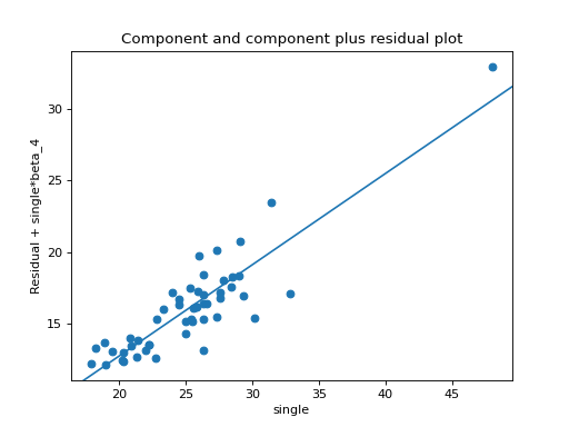
Generates a component and component-plus-residual (CCPR) plot.

Parameters:

resultsresult instance: A regression results instance.
exog_idx{int, str}: Exogenous, explanatory variable. If string is given, it should be the variable name that you want to use, and you can use arbitrary translations as with a formula.
axAxesSubplot, optional: If given, it is used to plot in instead of a new figure being created.

Returns:

Figure: If ax is None, the created figure. Otherwise the figure to which ax is connected.

See also

plot_ccpr_grid: Creates CCPR plot for multiple regressors in a plot grid.

Notes

The CCPR plot provides a way to judge the effect of one regressor on the response variable by taking into account the effects of the other independent variables. The partial residuals plot is defined as Residuals + B_i*X_i versus X_i. The component adds the B_i*X_i versus X_i to show where the fitted line would lie. Care should be taken if X_i is highly correlated with any of the other independent variables. If this is the case, the variance evident in the plot will be an underestimate of the true variance.

References

http://www.itl.nist.gov/div898/software/dataplot/refman1/auxillar/ccpr.htm

Examples

Using the state crime dataset plot the effect of the rate of single households (‘single’) on the murder rate while accounting for high school graduation rate (‘hs_grad’), percentage of people in an urban area, and rate of poverty (‘poverty’).

>>> import statsmodels.api as sm
>>> import matplotlib.pyplot as plot
>>> import statsmodels.formula.api as smf

>>> crime_data = sm.datasets.statecrime.load_pandas()
>>> results = smf.ols('murder ~ hs_grad + urban + poverty + single',
...                   data=crime_data.data).fit()
>>> sm.graphics.plot_ccpr(results, 'single')
>>> plt.show()

(Source code, png, hires.png, pdf)