Trends and cycles in unemployment

Here we consider three methods for separating a trend and cycle in economic data. Supposing we have a time series $y_t$, the basic idea is to decompose it into these two components:

$$y_t={\mu }_t+{\eta }_t$$

where ${\mu }_t$ represents the trend or level and ${\eta }_t$ represents the cyclical component. In this case, we consider a stochastic trend, so that ${\mu }_t$ is a random variable and not a deterministic function of time. Two of methods fall under the heading of “unobserved components” models, and the third is the popular Hodrick-Prescott (HP) filter. Consistent with e.g. Harvey and Jaeger (1993), we find that these models all produce similar decompositions.

This notebook demonstrates applying these models to separate trend from cycle in the U.S. unemployment rate.

%matplotlib inline

import numpy as np
import pandas as pd
import statsmodels.api as sm
import matplotlib.pyplot as plt

from pandas_datareader.data import DataReader
endog = DataReader('UNRATE', 'fred', start='1954-01-01')
endog.index.freq = endog.index.inferred_freq

Hodrick-Prescott (HP) filter

The first method is the Hodrick-Prescott filter, which can be applied to a data series in a very straightforward method. Here we specify the parameter $\lambda =129600$ because the unemployment rate is observed monthly.

hp_cycle, hp_trend = sm.tsa.filters.hpfilter(endog, lamb=129600)

Unobserved components and ARIMA model (UC-ARIMA)

The next method is an unobserved components model, where the trend is modeled as a random walk and the cycle is modeled with an ARIMA model - in particular, here we use an AR(4) model. The process for the time series can be written as:

$$\begin{array}{r}\begin{array}{rl}{y}_t& ={\mu }_t+{\eta }_t\\ {\mu }_{t+1}& ={\mu }_t+{ϵ}_{t+1}\\ \varphi (L){\eta }_t& ={\nu }_t\end{array}\end{array}$$

where $\varphi (L)$ is the AR(4) lag polynomial and ${ϵ}_t$ and ${\nu }_t$ are white noise.

mod_ucarima = sm.tsa.UnobservedComponents(endog, 'rwalk', autoregressive=4)
# Here the powell method is used, since it achieves a
# higher loglikelihood than the default L-BFGS method
res_ucarima = mod_ucarima.fit(method='powell', disp=False)
print(res_ucarima.summary())

                        Unobserved Components Results
==============================================================================
Dep. Variable:                 UNRATE   No. Observations:                  825
Model:                    random walk   Log Likelihood                -458.267
                              + AR(4)   AIC                            928.535
Date:                Wed, 02 Nov 2022   BIC                            956.820
Time:                        17:11:00   HQIC                           939.386
Sample:                    01-01-1954
                         - 09-01-2022
Covariance Type:                  opg
================================================================================
                   coef    std err          z      P>|z|      [0.025      0.975]
--------------------------------------------------------------------------------
sigma2.level     0.0784      0.168      0.466      0.641      -0.251       0.408
sigma2.ar        0.0980      0.171      0.574      0.566      -0.236       0.432
ar.L1            1.0638      0.116      9.203      0.000       0.837       1.290
ar.L2           -0.1799      0.327     -0.551      0.582      -0.820       0.460
ar.L3            0.0916      0.199      0.461      0.645      -0.298       0.481
ar.L4           -0.0214      0.082     -0.260      0.795      -0.183       0.140
===================================================================================
Ljung-Box (L1) (Q):                   0.00   Jarque-Bera (JB):           6101480.12
Prob(Q):                              0.95   Prob(JB):                         0.00
Heteroskedasticity (H):               9.36   Skew:                            17.14
Prob(H) (two-sided):                  0.00   Kurtosis:                       423.16
===================================================================================

Warnings:
[1] Covariance matrix calculated using the outer product of gradients (complex-step).

Unobserved components with stochastic cycle (UC)

The final method is also an unobserved components model, but where the cycle is modeled explicitly.

$$\begin{array}{r}\begin{array}{rl}{y}_t& ={\mu }_t+{\eta }_t\\ {\mu }_{t+1}& ={\mu }_t+{ϵ}_{t+1}\\ {\eta }_{t+1}& ={\eta }_t\cos {\lambda }_{\eta }+{\eta }_t^{\ast }\sin {\lambda }_{\eta }+{\tilde{\omega }}_t& {\tilde{\omega }}_t\sim N(0,{\sigma }_{\tilde{\omega }}^2)\\ {\eta }_{t+1}^{\ast }& =-{\eta }_t\sin {\lambda }_{\eta }+{\eta }_t^{\ast }\cos {\lambda }_{\eta }+{\tilde{\omega }}_t^{\ast }& {\tilde{\omega }}_t^{\ast }\sim N(0,{\sigma }_{\tilde{\omega }}^2)\end{array}\end{array}$$

mod_uc = sm.tsa.UnobservedComponents(
    endog, 'rwalk',
    cycle=True, stochastic_cycle=True, damped_cycle=True,
)
# Here the powell method gets close to the optimum
res_uc = mod_uc.fit(method='powell', disp=False)
# but to get to the highest loglikelihood we do a
# second round using the L-BFGS method.
res_uc = mod_uc.fit(res_uc.params, disp=False)
print(res_uc.summary())

                            Unobserved Components Results
=====================================================================================
Dep. Variable:                        UNRATE   No. Observations:                  825
Model:                           random walk   Log Likelihood                -461.552
                   + damped stochastic cycle   AIC                            931.103
Date:                       Wed, 02 Nov 2022   BIC                            949.950
Time:                               17:11:00   HQIC                           938.334
Sample:                           01-01-1954
                                - 09-01-2022
Covariance Type:                         opg
===================================================================================
                      coef    std err          z      P>|z|      [0.025      0.975]
-----------------------------------------------------------------------------------
sigma2.level        0.1419      0.022      6.416      0.000       0.099       0.185
sigma2.cycle        0.0279      0.021      1.344      0.179      -0.013       0.069
frequency.cycle     0.3491      0.206      1.698      0.090      -0.054       0.752
damping.cycle       0.7710      0.068     11.386      0.000       0.638       0.904
===================================================================================
Ljung-Box (L1) (Q):                   1.72   Jarque-Bera (JB):           6215485.79
Prob(Q):                              0.19   Prob(JB):                         0.00
Heteroskedasticity (H):               9.34   Skew:                            17.32
Prob(H) (two-sided):                  0.00   Kurtosis:                       427.59
===================================================================================

Warnings:
[1] Covariance matrix calculated using the outer product of gradients (complex-step).

/opt/hostedtoolcache/Python/3.10.8/x64/lib/python3.10/site-packages/statsmodels/base/model.py:604: ConvergenceWarning: Maximum Likelihood optimization failed to converge. Check mle_retvals
  warnings.warn("Maximum Likelihood optimization failed to "

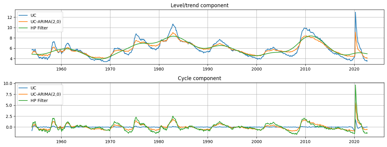
Graphical comparison

The output of each of these models is an estimate of the trend component ${\mu }_t$ and an estimate of the cyclical component ${\eta }_t$. Qualitatively the estimates of trend and cycle are very similar, although the trend component from the HP filter is somewhat more variable than those from the unobserved components models. This means that relatively mode of the movement in the unemployment rate is attributed to changes in the underlying trend rather than to temporary cyclical movements.

fig, axes = plt.subplots(2, figsize=(13,5));
axes[0].set(title='Level/trend component')
axes[0].plot(endog.index, res_uc.level.smoothed, label='UC')
axes[0].plot(endog.index, res_ucarima.level.smoothed, label='UC-ARIMA(2,0)')
axes[0].plot(hp_trend, label='HP Filter')
axes[0].legend(loc='upper left')
axes[0].grid()

axes[1].set(title='Cycle component')
axes[1].plot(endog.index, res_uc.cycle.smoothed, label='UC')
axes[1].plot(endog.index, res_ucarima.autoregressive.smoothed, label='UC-ARIMA(2,0)')
axes[1].plot(hp_cycle, label='HP Filter')
axes[1].legend(loc='upper left')
axes[1].grid()

fig.tight_layout();